6.3. Example: Tumurbulag Soum simulation calculation
Here is an example of how to do a simulation in Jupyter, using the calculation of Tumurbulag Soum.
6.3.1. Data preparation and computation
import pysd
import numpy as np
import pandas as pd
import re
from pathlib import Path
import matplotlib.pyplot as plt

import warnings
warnings.filterwarnings('ignore')
Define three scenario simulation parameters.
keys = ['Forage production','Carrying capacity','Livestock','Livestock output','Livestock output rate']
Define functions to compute for multi-scenario simulations.
def calculate(project_path):

    historical_livestock = pd.read_excel( project_path / 'input_data.xlsx',
                                         'historical_livestock').iloc[1][2:].values.astype('float')
    for scenario in [126,245,585]:
        fn = project_path / 'models' / f'{scenario}.py'
        strings = open(fn).read()
        modified_string = re.sub(r',\n    lambda: (\d+)', r',\n    lambda: '+str(int(historical_livestock[0])), strings)
        open(fn,'w',encoding='utf-8').write(modified_string)

    x = np.log(np.arange(1,historical_livestock.shape[0]+1))
    BAUk,BAUb = np.polyfit(x,historical_livestock,1)
    x = np.arange(36)

    BAU_values = BAUk*np.log(x)+BAUb

    all_results = []
    for scenario in [126,245,585]:
        model = pysd.load( project_path / 'models' / f'{scenario}.py' )
        all_results.append(model.run()[keys])
    for key in keys:
        all_results[0][key].iloc[7] = all_results[1].iloc[7][key]
        all_results[1][key].iloc[7] = all_results[1].iloc[7][key]
        all_results[2][key].iloc[7] = all_results[1].iloc[7][key]

    all_results[0]['Livestock'].iloc[7] = historical_livestock[-1] # 126
    all_results[1]['Livestock'].iloc[7] = historical_livestock[-1] # 245
    all_results[2]['Livestock'].iloc[7] = historical_livestock[-1] # 585

    return all_results,BAU_values
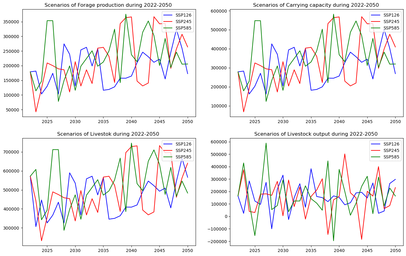
6.3.2. Livestock systems scenarios, 2022-2050
project_path = Path('Tumurbulag')
all_results,  BAU_values = calculate(project_path)
results = [i[7:] for i in all_results]
Define functions to graph the simulated data.
def show_results(results):
    colors = ['blue','red','green']
    plt.figure(figsize=(16,10))
    plt.subplot(2,2,1)
    for i in range(3):
        plt.plot(np.arange(2022,2051),results[i]['Forage production'].values,colors[i])
        plt.legend(['SSP126','SSP245','SSP585'],loc='upper right')
    plt.title('Scenarios of Forage production during 2022-2050 ')

    plt.subplot(2,2,2)
    for i in range(3):
        plt.plot(np.arange(2022,2051),results[i]['Carrying capacity'].values,colors[i])
        plt.legend(['SSP126','SSP245','SSP585'],loc='upper right')
    plt.title('Scenarios of Carrying capacity during 2022-2050 ')

    plt.subplot(2,2,3)
    for i in range(3):
        plt.plot(np.arange(2022,2051),results[i]['Livestock'].values,colors[i])
        plt.legend(['SSP126','SSP245','SSP585'],loc='upper right')
    plt.title('Scenarios of Livestok during 2022-2050 ')

    plt.subplot(2,2,4)
    for i in range(3):
        plt.plot(np.arange(2022,2051),results[i]['Livestock output'].values,colors[i])
        plt.legend(['SSP126','SSP245','SSP585'],loc='upper right')
    plt.title('Scenarios of Livestock output during 2022-2050 ')
show_results(results)
Define a function to compute the regulation parameters:
def scen(results):
    means = []
    stds = []
    MV = []
    SV = []
    for key in keys:
        mean_ = np.array([re[key].mean() for re in results])
        MV.extend(mean_)
        std_ = np.array([re[key].std() for re in results])
        SV.extend(std_)
        means.append((mean_==(mean_.max()))+(mean_==(mean_.min()))*-1)
        stds.append((std_==(std_.min()))+(std_==(std_.max()))*-1)
    MV.extend([np.nan]*3)
    SV.extend([np.nan]*3)

    index = pd.MultiIndex.from_product(
        [["Forage production/ton", "Carrying capacity/SU","Livestock/SU","Livestock output/SU","Livestock output rate/SU","Sustainability scores"],
         ["SSP126", "SSP245", "SSP585"]],
        names=["Variable", "Scenarios"]
    )

    columns = ["MV", "SV", "MV'", "SV'", "TV_j"]

    MV_ = np.concatenate([np.array(means).flatten(),np.array(means).sum(axis=0)])
    SV_ =np.concatenate([np.array(stds).flatten(),np.array(stds).sum(axis=0)])
    TV = MV_+SV_
    data = np.concatenate([[MV],[SV],[MV_],[SV_],[TV]])
    Sus_df = pd.DataFrame(data.T, index=index, columns=columns)
    return Sus_df, means, stds
Perform the calculations and view the results:
Sus_df,means, stds = scen(results)
Sus_df
Define the function to compute the modulation result:
def show_text():

    TV = np.array(means).sum(axis=0)+np.array(stds).sum(axis=0)
    if TV[1]>=2:
        SSP_index=1
    else:
        SSP_index = np.argmax(TV)
    Best_Scenario = 'SSP'+str([126,245,585][SSP_index])

    text = f"""Best Scenario is {Best_Scenario}.
    Over the next three decades, forage production, carrying capacity, livestock numbers and livestock output fluctuate and remain stable.
    Among the three scenarios (SSP126, SSP245 and SSP585),the {Best_Scenario} scenario for {project_path.name} in the lower reaches of the basin,
    was identified as the rational scenario for the highest productivity and stability.
    """
    print(text)
    return SSP_index, Best_Scenario
Run the above function:
SSP_index, Best_Scenario = show_text()
Best Scenario is SSP126.
    Over the next three decades, forage production, carrying capacity, livestock numbers and livestock output fluctuate and remain stable.
    Among the three scenarios (SSP126, SSP245 and SSP585),the SSP126 scenario for Tumurbulag in the lower reaches of the basin,
    was identified as the rational scenario for the highest productivity and stability.
6.3.3. Changes in stock ratio between historical and forecast periods
Define the function and compute the change :
def change():
    historical_data = pd.read_excel(project_path / 'input_data.xlsx','grassland_area').iloc()[SSP_index+1][2:9]
    grass_land_area = np.nanmean(historical_data.values)

    Carrying_capacity_Scenario = Sus_df['MV']['Carrying capacity/SU'][SSP_index]
    Forage_production_Scenario = Sus_df['MV']['Forage production/ton'][SSP_index]
    Livestock_Scenario = Sus_df['MV']['Livestock/SU'][SSP_index]
    Livestock_output_Scenario = Sus_df['MV']['Livestock output/SU'][SSP_index]

    Forage_production_before = all_results[SSP_index][:8]['Forage production'].mean()
    Carrying_capacity_before = all_results[SSP_index][:8]['Carrying capacity'].mean()
    Livestock_before = all_results[SSP_index][:8]['Livestock'].mean()
    Livestock_output_before = all_results[SSP_index][:8]['Livestock output'].mean()


    data = [[project_path.name,
             '2015-2022',
             '%d'%(Forage_production_before/grass_land_area*1000),
             '%d' %(Carrying_capacity_before),
             '%.2f'%(Carrying_capacity_before/grass_land_area),
             '%d'%(Livestock_before),'%.2f'%(Livestock_before/Carrying_capacity_before),
             '%d'%(Livestock_output_before)],
            ['',
             '2022-2050',
             '%d'%(Forage_production_Scenario/grass_land_area*1000),
             '%d' %(Carrying_capacity_Scenario),
             '%.2f'%(Carrying_capacity_Scenario/grass_land_area),
             '%d'%(Livestock_Scenario),
             '%.2f'%(Livestock_Scenario/Carrying_capacity_Scenario),
             '%d'%(Livestock_output_Scenario)]
           ]

    # Define indexes for multiple layers of columns
    columns = pd.MultiIndex.from_tuples([
        ('Soums', ''),
        ('Period', ''),
        ('Grassland', 'Forage (kg/ha)'),
        ('Grassland', 'Carrying capacity (SU)'),
        ('Grassland', 'Carrying capacity (SU/ha)'),
        ('Livestock', 'Livestock (SU)'),
        ('Livestock', 'Stocking rate'),
        ('Livestock', 'Livestock output (SU)')
    ])
    change_df = pd.DataFrame(data, columns=columns)

    num1 = (Forage_production_Scenario-Forage_production_before)*100/Forage_production_before
    num2 = Carrying_capacity_before/grass_land_area
    num3 = Carrying_capacity_Scenario/grass_land_area
    num4 = Livestock_before/Carrying_capacity_before
    num5 = Livestock_Scenario/Carrying_capacity_Scenario
    text = f'''The projected average forage yield in {project_path.name} is expected to {'increase' if num1 > 0 else'decrease'} by {'%.2f'%(abs(num1))}%,
    compared to the historical period.
    The carrying capacity is projected to {'decrease' if num2<num3 else 'increase'} from {'%.2f'%num2} SU/ha during 2015-2022 to {'%.2f'%num3} SU/ha during 2022-2050.
    The stocking rate is projected to {'decrease' if num4<num5 else 'increase'} from {'%.2f'%num4} during 2015-2022 to {'%.2f'%num5} during 2022-2050.'''
    print(text)
    return change_df
Run the function to generate the result:
change_df = change()
The projected average forage yield in Tumurbulag is expected to increase by 0.67%,
    compared to the historical period.
    The carrying capacity is projected to decrease from 1.19 SU/ha during 2015-2022 to 1.21 SU/ha during 2022-2050.
    The stocking rate is projected to decrease from 1.46 during 2015-2022 to 1.55 during 2022-2050.
change_df
6.3.4. Regression simulation of livestock systems
Define functions to compute strategy recommendations based on the results of the scenario simulation.
def strategy():
    BAU = BAU_values[8:].mean()
    Cp = results[SSP_index].mean()['Carrying capacity']
    stock_rate_BAU = BAU/Cp
    SSP_RCP_Scenarios = results[SSP_index].mean()['Livestock']
    Stock_rate_Scenario = SSP_RCP_Scenarios/Cp
    BAU_RCP_Reduction = BAU-SSP_RCP_Scenarios
    reduction_rate_0 = BAU_RCP_Reduction/BAU
    RCP_Cp_Reduction = SSP_RCP_Scenarios-Cp
    reduction_rate_1 = RCP_Cp_Reduction/SSP_RCP_Scenarios

    columns = "Livestock    BAU     SSP-RCP Scenarios       Carrying capacity       Reduction from BAU to rational scenarios        Reduction rate from BAU to rational scenarios   Reduction from scenarios to Carrying capacity   Reduction rate from scenarios to Carrying capacity ".split('\t')
    data = [project_path.name,BAU,SSP_RCP_Scenarios,Cp,BAU_RCP_Reduction,reduction_rate_0,RCP_Cp_Reduction,reduction_rate_1]
    strategy_df = pd.DataFrame(np.array([data]), columns=columns)
    text = f"""In the coming three decades, {project_path.name} will be heavily overloaded under the BAU scenario,
    and even under the rational SSP scenarios.
    To maintain forage-livestock equilibrium,livestock should be reduced in the two consecutive steps:
    1) First Step:reducing livestock from BAU torational future scenarios by {'%d' %BAU_RCP_Reduction} SU ({'%.2f' %(reduction_rate_0*100)}% reduction).
    2) SecondStep: reducing livestock from rational scenarios to carrying capacity {'%d' %RCP_Cp_Reduction} SU ({'%.2f' %(reduction_rate_1*100)}% reduction)."""
    print(text)

    return strategy_df
Run the function and see the results:
strategy_df = strategy()
strategy_df
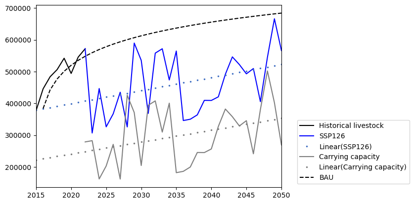
In the coming three decades, Tumurbulag will be heavily overloaded under the BAU scenario,
    and even under the rational SSP scenarios.
    To maintain forage-livestock equilibrium,livestock should be reduced in the two consecutive steps:
    1) First Step:reducing livestock from BAU torational future scenarios by 171060 SU (26.89% reduction).
    2) SecondStep: reducing livestock from rational scenarios to carrying capacity 164164 SU (35.31% reduction).
Define the function, fit it, and plot it:
def plot_fit():
    historical_livestock = pd.read_excel( project_path / 'input_data.xlsx',
                                         'historical_livestock').iloc[1][2:].values.astype('float')
    plt.plot(np.arange(2015,2023),historical_livestock,color='black')
    plt.plot(np.arange(2022,2051),results[SSP_index]['Livestock'].values,color='#0000FF')
    x,y = [np.arange(2022,2051),results[SSP_index]['Livestock'].values]
    k,b = np.polyfit(x,y,1)

    print(k,b)

    plt.plot(np.arange(2015,2051),k*np.arange(2015,2051)+b,'.',color='#4472C4',markersize=3)
    x,y = [np.arange(2022,2051),results[SSP_index]['Carrying capacity'].values]
    k,b = np.polyfit(x,y,1)
    print(k,b)

    plt.plot(x,y,color='#7F7F7F')
    plt.plot(np.arange(2015,2051),k*np.arange(2015,2051)+b,'.',color='#7F7F7F',markersize=3)
    plt.plot(np.arange(2015,2051),BAU_values,'--',c='black')
    plt.xlim(2015,2050)
    plt.legend(['Historical livestock',Best_Scenario,f'Linear({Best_Scenario})','Carrying capacity','Linear(Carrying capacity)','BAU'],
               bbox_to_anchor=(1.05,0),
               loc='lower left')
Run this function:
plot_fit()
4104.998173025084 -7892787.658744299
3737.161682109544 -7308037.384229856